Documentation
How it works
This is the long version. If you only want to know what the integration does and how to set it up, stay in the README — it has a one-page summary of the same loop. This document is for when a plan surprised you and you want to know why, or when you are deciding whether a setting is worth turning on.
Everything below describes the code in this repository. Where a number is a default, it is the default the code ships; where a figure came from a measurement, it says so.
What the optimizer is actually solving
A heat pump has one job — keep the house at a temperature you like — and almost no freedom in when it does it, because most controllers only react to the room they are standing in. But a house is a thermal store. Heat bought at 02:00 is still largely there at 08:00, and electricity at 02:00 can cost a fraction of what it costs at 08:00. The same is true of a hot water tank, only more so: nobody notices what time the water was heated.
So the question the optimizer answers is not "should the pump run now" but:
Given the prices I can see, the weather I expect, and what I know about how this particular house holds heat — what is the cheapest schedule for the next 24 hours that still keeps every room inside its comfort band and hot water available when it is wanted?
That is a model predictive control (MPC) problem, and it needs three things to be right: a forecast (prices, temperature, wind, rain, sun), a model of how this house turns electricity into indoor temperature and loses it again, and an objective that says what "best" means — including what a degree of discomfort is worth in money.
The model is the part nobody can hand you. A datasheet describes a house that does not exist; yours has its own leakage, its own solar aperture, its own occupancy heat. So the model is learned, continuously, from the difference between what it predicted and what actually happened — and most of the engineering here is about learning it safely.
The planning cycle
Every optimization interval (30 minutes by default), the coordinator gathers inputs, builds a 24-hour horizon on a 15-minute grid, solves it, and publishes the result. Only the first step is ever acted on: the rest is re-solved next interval against fresher data. That is what makes an imperfect forecast survivable — a wrong guess about hour 20 is corrected forty times before hour 20 arrives.
sequenceDiagram
    autonumber
    participant C as Coordinator
    participant P as Prices (Tibber + learned prior)
    participant W as Weather entity (HA)
    participant S as Your sensors
    participant M as Thermal model
    participant O as Optimizer (MPC)
    participant E as Entities & card

    Note over C: every optimization interval (default 30 min)
    C->>P: published hourly prices
    P-->>C: prices + estimated tail (weekday/weekend prior,<br/>never displacing published data)
    C->>W: temperature, wind, rain, forecast irradiance
    Note over W: irradiance has three sources, in order:<br/>a local irradiance sensor, then Open-Meteo when<br/>selected (the only minutely_15 request),<br/>else this entity's own forecast
    C->>S: indoor/outdoor temps, tank temps, power
    S-->>C: staleness check → Input Problem sensor,<br/>learners freeze on bad input
    C->>M: build forecast arrays (24 h, 15-minute steps)
    M-->>O: predicted heat demand, COP, solar gain,<br/>DHW draw quantiles
    O->>O: solve: hot water first (LP + repair),<br/>then space heating around it,<br/>then one co-optimization pass
    O-->>C: space + DHW slot plan
    C->>C: apply manual-plan pins (≤20 h),<br/>safety releases pinned-off slots
    C->>E: publish plan sensors, switch heat pump,<br/>ECL110 displace / frequency advice
    Note over C: between plans the peak guard folds power-meter events<br/>and flips a flag (2 agree engage / 2 clear).<br/>It never solves — the next solve only reads the flag
    Note over M: afterwards: compare prediction vs reality,<br/>nudge learned parameters
Why hot water is solved first. The two circuits share one compressor but are very different problems. Space heating is continuous with a smooth objective, so a gradient solver handles it well. Hot water is an on/off block load with hard deadlines, which a gradient solver smears into a trickle the hardware cannot deliver. So hot water is planned first — a linear program plus repair passes against the real tank simulation — and space heating is then optimized around the fixed DHW blocks by multi-start L-BFGS-B.
Solving them in sequence would let hot water fill the cheapest hours to the compressor ceiling and push space heating into dearer ones. Two things prevent that:
- A congestion premium inside the DHW program. Taking compressor capacity in a step where space heating also wants it is charged the extra price of buying the displaced space heating elsewhere, using the cheapest step with spare capacity within a 6-hour window either side. Beyond a few hours the building has already lost the heat, so a cheap hour tomorrow is not a substitute for a shortfall this morning.
- One co-optimization pass. Once the space profile is known, hot water is re-planned against it — but the second plan is adopted only if it scores strictly better on the same objective. That is what makes a single extra iteration safe instead of something that has to run to convergence.
Without the premium, hot water displaced 2.6–4.7 kWh of space heating into more expensive hours in the validation scenarios.
Several starting points, not one. A single gradient run can stop at a locally optimal schedule that a different starting guess beats — that is what the two-zone model showed. So each space solve scores four candidate profiles cheaply (a warm start or the naive guess, two price-ranked profiles at different total energy, and a flat half-headroom guess), refines every one of them with L-BFGS-B, and keeps whichever refinement scores best. Four candidates close most of the local-optimum gap in the two-zone model; a fifth would not be worth the extra full solve on the hardware Home Assistant runs on.
The objective, term by term
What the space heating solve minimizes:
| Term | What it prices |
|---|---|
grid_cost(P_space + P_dhw) |
Electricity, piecewise in PV surplus, × price_weight |
| comfort terms | Pull toward the target, plus penalties for breaching the floor/ceiling |
| cycling cost | Compressor start-stop wear, × price_weight |
| capacity tariff | The month's peak charge exposure, × price_weight |
| terminal cost | The value of heat left stored at the end of the horizon |
Every term except the comfort penalties is denominated in money. The comfort
terms are the exchange rate between money and warmth, and comfort_weight
(default 5) is the dial that sets it.
Comfort bounds are soft, not hard. A hard band could make a cold morning infeasible — there is no schedule that holds 19 °C if the pump cannot deliver it — and an infeasible problem produces no plan at all. So breaching the floor is expensive rather than forbidden. The floor penalty is quadratic plus a small linear term: a purely quadratic penalty has vanishing gradient at the boundary, so the solver settles just under the floor where the breach costs almost nothing and the electricity saved is worth real money. The linear term gives the penalty a non-zero slope at the boundary and pins the trajectory to the floor instead.
The pull toward the target is deliberately weak. Twice the strength, on the winter scenario, makes the plan spend 28.55 SEK instead of 23.28 — 18% of the bill — buying an average 0.32 K of extra warmth while never coming near the floor. Below the chosen strength the saving plateaus, so it sits where the money stops improving and a real preference is still expressed.
Money terms scale with price_weight together. If the energy cost scaled
and the cycling and capacity terms did not, a non-default price weight would
silently re-price compressor starts and grid peaks against the electricity they
trade off.
There is no smoothness term. A 0.01 · Σ ΔP² smoothness regulariser
would be priced in invented units, and measured, it costs about 5% of the
two-zone winter bill for no reduction in compressor starts. Discouraging
chatter is the cycling cost's job, and that is denominated in currency per
start-stop cycle.
Weather anticipation is emergent, not a bonus
There is no "heat before the wind arrives" term and no "don't heat before the sun" term. The trajectory simulation applies forecast solar gain and the wind/rain heat-loss factors to the real dynamics at every future step. A plan that pre-heats the slab before a sunny morning therefore predicts an overheated house and gets charged for the electricity it wasted; a plan that coasts into a windy evening predicts a cold house and a comfort penalty. Both are avoided because they are genuinely more expensive.
The objective carries no separate anticipation term on top of this. Such a term would count physics the simulation already has a second time, and a weather bonus is a negative cost: it pays the plan to burn electricity before bad weather. The solar forecast also shapes the solver's initial guess, where a wrong hunch costs nothing.
The terminal cost, and why it needs caps
Nothing beyond the horizon is scored, so without a terminal term the optimizer
dumps the last couple of hours: it coasts the house down because the resulting
cold never appears in the objective. That breaches comfort at the tail of the
plan and reports a saving that was really borrowed heat. So the heat each
store is short of at the horizon's end is priced against the same reference the
savings settlement uses — the 25th-percentile price, scaled by price_weight.
Each store converts at its own marginal COP. ThermalModel.marginal_cop
is the single answer to "what does one more kWh into this store cost", shared
by the trajectory simulation and by every terminal and deferred valuation:
- building mass (room, slab, upper, lower) heats at the plain space curve;
- the buffer tank charges at the flow-derated COP of the tank's own temperature;
- the DHW tank charges at
compute_cop_dhwat the tank's temperature: the buffer's own flow-derated law, on every plant, so the two tanks cost the same per kWh at the same water temperature. A tank below the reference flow (cop_flow_reference_temp, 35 °C by default) earns no boost.
Each is priced at the forecast humidity: the step's own where the plan buys heat, and the horizon's mean where a valuation prices at the mean outdoor temperature. The planner and the published trajectory therefore read the same humidity, so the defrost derate cannot plan hot water at one humidity and deliver it at another.
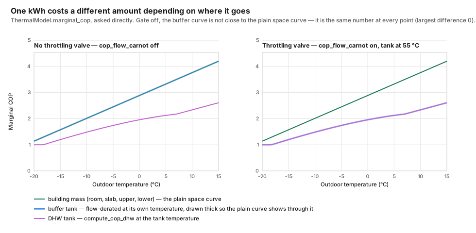
Both panels are marginal_cop asked directly over the same outdoor range. With
the gate off, the buffer and building-mass curves are not merely close — the
generator measures their largest difference and prints it, and it is zero.
The sharing matters. A simulation charging a throttled buffer at the derated
COP while the settlement terms paid every stored kWh back at the plain curve
would put marginal value below marginal cost, which is systematic
under-charging: the solver would store heat only when the price spread also
covered a COP gap the physics never charged. The buffer derate is gated on cop_flow_carnot, so installs with
no throttling valve return the plain curve bit for bit.
Settlement caps stop the reverse error — being paid for heat nobody needs:
-
Room is capped at the comfort target, not the ceiling. A house sitting at 25 °C in July because the sun heated it is not holding 4 °C of useful charge, and settling that up would charge the plan for failing to be as overheated as the reference.
-
Slab is capped at the temperature that sustains the target in steady state — it has to run above the room to push heat into it. In two-zone mode that demand is sized from the lower zone alone, because the slab feeds only the lower zone (the upper zone is radiator-fed) and it uses the lower zone's share of internal gains. Sizing it from the whole house would inflate the cap by the upper zone's demand and over-value hot-slab end states by exactly that much.
-
Buffer gets a much higher cap, because that reasoning does not transfer to a tank: a tank only gets hot because the pump deliberately heated it, so every degree in it will be used. The slab's cap would make the tank invisible — charging from 45 °C to 70 °C would be credited with 0.0 kWh of the 21.8 kWh actually stored, so charging would be pure cost and every plan would collapse to no storage.
The buffer cap is the ceiling the plan can actually charge to, not the raw safety rating. Reaching the rating requires the pump to out-run the house's standing draw and the tank's own standby loss at an ever-worsening flow-derated COP, which in cold weather a real pump cannot. The ceiling is found by bisection on the net charge rate (monotone decreasing in tank temperature) and lands on the rating in every mild-weather case. The learned house-leakage scale rides along, because without it a learned-leaky house would get an optimistic ceiling — the one direction this bound must not err.
The cap is then floored at the tank temperature the solve started from, clipped at the rating. Heat already in the tank above the charging ceiling is real: it was paid for, and draining it displaces bought electricity. Capping at the ceiling alone would let a plan drain a pre-charged tank — a mild evening's 60 °C ahead of a cold snap — with zero settlement, re-creating the tail-dumping this term exists to prevent in exactly the regime where storage matters most.
-
Wood tank, when modelled as its own store, is settled up to 95 °C — but only in the reported figures, never in the objective. Nobody refills a wood tank with electricity, so crediting it in the objective would create a hoarding incentive with no refill cost.
The thermal model
One zone or two
With only a house thermal mass and a heat loss coefficient configured, the model is single-zone: one room temperature, one slab, one buffer tank. Two-zone mode adds a second room temperature and a transfer coefficient between them, and is the right model for the common Nordic house — a slab-heated lower floor and radiators upstairs.
flowchart TB
    hp["Heat pump<br/>(COP from outdoor temp,<br/>flow temp, defrost derate)"] --> buf["Buffer tank"]
    buf -- "radiator share<br/>(default 40%)" --> up["Upper zone<br/>low mass, fast"]
    buf -- "floor share<br/>(default 60%)" --> slab["Slab<br/>high mass, slow"]
    slab --> low["Lower zone"]
    up -- "inter-zone transfer<br/>(open layout)" --- low
    sun["Solar gain<br/>40% upper / 60% lower"] --> up
    sun --> low
    up --> out["Outdoors<br/>wind ↑ convective loss<br/>rain ↑ envelope U"]
    low --> out
    buf --> out
The two zones are not symmetric and that is the point: the upper zone is light and responds within the hour, the slab holds heat for most of a day. A plan that pre-charges the slab overnight and coasts the radiators through a morning peak is only visible to a model that knows they are different.
Defaults, for orientation: upper mass 3 kWh/°C, lower 8 kWh/°C, upper loss 0.08 kW/°C, lower 0.07 kW/°C, inter-zone transfer 0.5 kW/°C, radiator share 0.4, buffer tank 35 L. Single-zone defaults are a 10 kWh/°C house at 0.15 kW/°C. When two-zone parameters are not configured the model falls back to single-zone; hot water optimization activates as soon as any one of a DHW temperature sensor, a tank volume or a set of demand windows is configured.
Heat loss, wind and rain
Heat loss is recomputed at every forecast step, not once per plan:
U_effective = U_base × house_heat_loss_scale
            × (1 + wind_sensitivity × wind_speed)
            × rain_multiplier   (when it is raining)
Wind (default 0.03, i.e. +3% per m/s) models infiltration and convective loss; only the infiltration share of the loss actually responds to wind, so the whole-house sensitivity is small. Measured infiltration studies put a 10 m/s wind at roughly +20–40% for typical tightness, which is what a draughty or exposed house should be tuned toward. Rain (default 1.15, +15%) models a wet envelope, scaled by intensity so light rain gives a partial multiplier. Ranges and per-house suggestions are in configuration.md.
There is an opt-in refinement: snow is not rain. The rain multiplier is weighted by the liquid fraction of forecast precipitation, and a second opt-in halves modelled solar gain for two days after heavy snowfall, because snow on the glazing blocks the sun the plan was counting on.
Solar gain
Q_solar = irradiance × window_area × orientation_factor × SHGC / 1000
split 40% upper / 60% lower by default in two-zone mode, on the reasoning that in an open layout the sun reaches the lower floor through large windows. Defaults: 10 m² glazing, orientation factor 0.7 (south-facing bias), SHGC 0.7 (typical double-glazed low-e).
Only the product of window area and SHGC is observable, which is why the learned solar aperture (below) scales the product rather than either factor.
Slab temperature from the floor return
With a floor heating return temperature sensor configured, the slab estimate is corrected toward the measurement each interval:
T_slab = 0.7 × (T_return + 1 °C) + 0.3 × T_slab_model
A floor circuit's return temperature is a good proxy for average slab temperature; the 70/30 merge keeps sensor noise out of a state variable the whole plan rests on.
Knowing the lower floor rather than guessing it
Two-zone mode plans against two room temperatures, and often only the upper one has a sensor. The floor return water is not used for the lower zone: a floor loop returns at roughly 24–30 °C while the room it serves sits near 21, so a water temperature standing in for an air temperature would make the lower floor read several degrees too warm, permanently overshooting its comfort band, and the optimizer would under-heat the one room it cannot see. The floor return keeps the job it is genuinely a proxy for — the slab estimate above — and the lower zone starts from the room sensor and is carried forward by the model's own dynamics. That is open-loop: nothing corrects it, so it can drift from the real downstairs over a long cold spell, and a repair notice says so rather than letting a modelled number pass for a measured one. The chart labels the trace "Lower floor (modelled)" until a thermometer is assigned.
Configuring a Lower floor temperature sensor closes the loop: the zone is measured, and slab-to-room becomes a real difference again. It is optional and two-zone only. The order of preference is a real sensor, then the room temperature.
Learning how the loss splits between the floors
Once a real lower-floor sensor exists, the split between the zones can stop
being taken on trust as well. The catch: house_heat_loss_scale, the correction
learned from prediction error, multiplies both zone losses. It can move the
total but never the split, so learning both zone losses independently alongside
it would be three parameters chasing two degrees of freedom — they trade off
against each other and drift without ever making the fit worse.
So the two get separate jobs. The scale owns the level and is fitted from
the upper floor; a ratio owns the split and is fitted from the lower floor,
which the scale's own fit does not touch. Two parameters, two independent
measurements. lower_floor_loss_ratio stays at 1.0 — the configured split —
until it has evidence.
Deliberately not learned: the inter-zone transfer coefficient. One pump, one water temperature and a fixed radiator/floor split mean the zones are driven together and rarely diverge, so a passive fit would mostly track noise.
The buffer tank as a store (mixing valve required)
Without a mixing valve, everything the heat pump makes goes straight to the radiators and floor loops. The buffer tank is then a hydraulic separator that happens to lose a little heat — whatever enters it leaves immediately, so it can never be charged. That is the default, and it is a correct model.
A mixing valve changes this: it limits how much heat reaches the house, so once the house has what it needs the surplus has nowhere to go but the tank. The Heating system and heat storage option offers four modes — no valve (default), a fixed valve you set by hand and declare, a valve read from a sensor but not written, and a valve commanded by the optimizer, which writes the target to a number or climate entity after each planning cycle and only when it changes.
A commanded valve can do something a hand-set one cannot: wait. A fixed valve starts feeding the house the moment the tank is warmer than its curve, so stored heat mostly gets used in the hours right after it was bought. Commanded, the plan can lower the valve's target between charging and the expensive hours — the house coasts on what the building itself holds, the tank keeps its heat — and raise it again for the peak. On the author's Swedish winter price curve that is worth roughly 1–2 SEK a day on top of what storage already saves; at flat prices the optimizer does not do it at all, because there is nothing to gain. The house is never planned below your comfort floor to achieve it.
What to set a hand-adjusted valve to: the top of your comfort band, in almost every case. A high setting keeps the valve open until the house reaches its ceiling, so the building charges first — and building storage is free, because the heat sits at room temperature. Only then does the valve throttle and the tank take the surplus, which is stored hot and does cost efficiency. Building first, tank second, is the cheap order. The cost of that choice is that the valve does not prevent the house overheating — the optimizer's comfort limits do.
Storing hot is not free. A heat pump loses efficiency the hotter it must push water, and that penalty is the whole economics of a thermal store: it decides whether moving heat into a cheap hour pays. The model accounts for it, so the tank is only charged when the price difference covers the loss, and never past the maximum you configure however cheap electricity gets.
A tank below 100 litres is not treated as a store at all, whatever the valve mode. The physics stay modelled, but the terminal credit and the settlement cap ignore it: a 35 L tank holds about 0.8 kWh over a 20 K swing, below the resolution of a single 15-minute step, while 100 L over a 30 K usable swing is about 3.5 kWh — a couple of hours of winter house load, and where a store starts to be able to move money.
Hot water
Hot water is a deferrable, essentially on/off load: the tank is a battery, and heat put in at any hour is still there later, minus standby loss.
Demand time frames
Hot water is only required during the time frames you configure — for example
06:00-08:30, 17:00-22:00. This is the single biggest lever on hot water cost.
- Inside a frame the tank is guaranteed to stay at or above the DHW minimum temperature (default 45 °C), so hot water is always available.
- When a frame opens the tank is pre-heated to a "ready" temperature sized from the draw actually expected in that frame plus its standby loss, clamped between the minimum and the configured setpoint. A household that uses little water is never heated to 55 °C just because the setpoint says so.
- Outside the frames there is no availability requirement at all. The tank drifts down, so no electricity is spent keeping water hot that nobody is going to use.
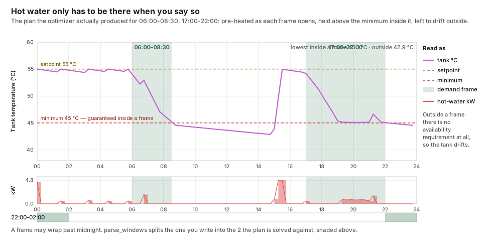
That figure is one the shipped optimizer produced rather than an illustration
of it: docs/img/model/make_model_figures.py reads the plan tests/plan_view.py
solved, shades the frames dhw_schedule.parse_windows returns for the spec
above, and refuses to write the figure at all if the plan it read dips below
the minimum inside a frame.
Frames accept 24-hour times separated by commas and may wrap past midnight
(22:00-02:00). A frame may also carry a day selector
(weekdays 06:00-08:30, weekend 08:00-09:30), and single weekdays can
override the schedule, so the requirement resolves per calendar day — the
grammar and its layers are configuration.md's to
document. Leave the field empty and the frames are derived from the
learned hourly usage profile instead. Switch the schedule off entirely to
require hot water around the clock.
Silent windows
Separate from the pump's own night-mode schedule (the options field labelled for that hardware fact), the card's Silent windows are your wish about noise. Each row is a day selector, start, end and an action: Silent caps the compressor in those hours; Off means the plan schedules no space heating and no hot-water slots in the window, with nothing extra written. An Off window may not overlap a hot-water demand frame on the same day; a Silent window may (the tank just charges slower). Switching the optimizer off inside a window undoes nothing.
How the schedule is produced
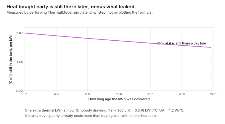
The decay above is not the formula below plotted; it is the shipped tank simulation perturbed by one kWh and asked what is left. That distinction is the point — a figure drawn from the formula would agree with this text however the model behaved.
Six passes, each fixing something the previous one cannot see:
-
A linear program over the whole horizon. The tank is a linear store, so its temperature at any step is an affine function of the heat put in earlier — a kWh delivered
ksteps ago still contributes(1 − UA·Δt/C)^k / Cdegrees today. MinimisingΣ price·energy/COPunder the availability floors and the tank maximum gives the cheapest feasible allocation. The decay factor is the standby loss, so buying early is automatically priced above buying late and no artificial "don't pre-heat more than N hours ahead" cap is needed — none is applied. Heating can land at 02:00 for a 17:00 frame whenever that is cheaper, subject only to what the tank can hold. A heavily-priced slack variable keeps the program feasible when the requirement simply cannot be met (a cold start, an undersized pump). -
A cheapest-first greedy pass repairs what the linear model got wrong — it ignores the COP's dependence on tank temperature and the cold-water floor — and takes over entirely if the solve is unavailable.
-
Minimum-run rounding. A DHW valve is on or off; a planned 0.05 kW trickle is not something the hardware can do. Each sub-minimum slot is raised if the tank stays within its rating and zeroed if raising it would boil the plan over. The decision is per slot: an all-or-nothing version gave up on every weak slot whenever raising them together would overshoot, and published a plan full of powers the hardware cannot run.
-
A second greedy pass re-buys the energy the zeroed slots were carrying.
-
The rating clamp walks the plan through the real tank simulation and truncates any step that would exceed the tank rating. This is physics, not preference, so it sits after the economics: no plan may boil the tank, however cheap the electricity.
-
The floor repair gives the floor the same physics check the rating just got. The LP and greedy passes plan on an affine tank; the trajectory the house actually runs is the simulation's, and the gap between them let a plan that satisfied every linear floor drain the real tank 1–2 °C below the promised minimum inside an evening demand frame. Each round simulates the whole plan, finds the first step whose simulated temperature breaches the requirement, sizes the missing electrical energy at the tank's own marginal COP, and adds it at the cheapest step with headroom that can still reach the breach — searching only after the last rating-pinned step before it, since heat added ahead of a full tank is refused rather than stored. Bounded at 48 rounds, so a demand no rating-legal plan can meet exits with the closest achievable trajectory instead of looping.
The repair's top-ups are deliberately not re-clamped afterwards. The external clamp predicts the tank without draw relief — conservative by design — so it reads in-frame top-ups, which exist precisely because the frame is draining the tank, as rating breaches and truncates them straight back out. The repair's own simulation runs the real step, whose internal rating clamp books any genuinely refused heat, so a repaired plan cannot overshoot where it matters.
The tank is never planned above min(70 °C, max(setpoint, legionella temp)).
What a draw actually costs the tank
The hourly draw pattern is stated as a nominal demand: the volume you use, heated from the cold-water inlet to the setpoint. That is exactly what a tank at or above the setpoint supplies, because mixing at the tap shrinks the drawn volume so the enthalpy removed stays nominal.
A colder tank cannot be debited energy referenced to a rise it does not hold. So the debit scales with the rise the tank can actually deliver, against a 40 °C mixed-use reference — the temperature water actually leaves a tap at:
q_effective = q_nominal × min(1, (T_tank - T_inlet) / (40 °C - T_inlet))
The tap draws more volume from a cooler tank to make the same mixed water, so
the enthalpy removed stays exactly nominal all the way down to 40 °C, and only
below that does the service itself degrade. Referencing the setpoint instead
would under-debit the 40 °C-to-setpoint band — the very band cost optimization
rides — by up to a third, and book the deleted demand as savings. Unscaled, a
30 °C tank would be charged the full (setpoint − inlet) per litre and the
inlet floor underneath would silently refund the fabricated deficit.
Demand-side quantities stay nominal on purpose: the planner's ready-energy targets and the always-hot baseline describe what you want delivered, and that does not shrink because the tank happens to be cold.
With the scaled draw, the inlet floor underneath is a genuine no-op safety bound, and any heat it does have to fabricate is booked rather than silently created. The default inlet reference is 10.0 °C; set Cold water inlet temperature on Hot water tank and inlet if you have measured yours.
Self-learning tank cooling
How far ahead pre-heating pays off depends entirely on how well the tank holds heat, so that is measured rather than assumed. The parameter is stated as a cooling rate in °C per hour at 45 °C tank temperature in a 20 °C room (default 0.3 °C/h) and converted to a UA value using the tank's thermal mass.
Every time the tank is sampled across an interval in which the heat pump did not run, the standby time constant follows from the decay itself:
UA/C = -ln((T_end - T_ambient) / (T_start - T_ambient)) / Δt
Hot water drawn during the interval can only make the tank look leakier than it is, never tighter, so observations are folded in as a lower envelope: the estimate moves quickly toward a quieter reading and only creeps upward. One shower cannot convince the model that the tank is badly insulated, while a genuinely deteriorating tank is still learned within a few days. The result is clamped to 0.05–3.0 °C/h and persisted across restarts, with the learned value, its sample count and the resulting hold time on the DHW Temperature sensor. A tank that holds heat well earns a longer pre-heating horizon; a leaky one is heated closer to when the water is needed.
The buffer tank rate uses the same estimator, but only when a buffer tank temperature sensor is configured. Without one, a prior derived from the tank's size is used — and both that prior and the range the learning may move within, follow the tank's surface area rather than its volume. Heat escapes through a tank's skin, and a large tank has far less skin for the water it holds: a 750-litre accumulator loses proportionally much less than a 35-litre buffer, so one "degrees per hour" figure cannot describe both. Applied unscaled, a small tank's figure models more heat lost in six hours than a big tank can physically hold, which makes storing heat in it look pointless when it is not.
Anti-legionella
Since the tank is allowed to cool between frames, a periodic disinfection cycle is enabled by default: every 7 days the tank is heated to 60 °C, scheduled at the cheapest hour before the deadline. The timer resets whenever the tank is observed at the disinfection temperature for any reason — planned cycle, manual boost, wood furnace, immersion heater — so an already-hot tank never triggers a redundant cycle.
Two opt-in refinements:
- Free disinfection: if another heat source holds the tank at the disinfection temperature long enough, that counts as a completed cycle. It is hold-verified, so a momentary blip at 60 °C credits nothing.
- A price-aware cycle: inside its interval the cycle may run a day or two early (no sooner than a configurable minimum, default 5 days) when a known price beats what a typical remaining day is expected to bottom out at. The deadline is always honoured; hygiene never waits for a better price.
Hot water that fits your household
Everything here is inert until configured or until evidence exists:
- The cold-water inlet is a setting, not an assumption — configurable, with an optional seasonal swing (coldest in late February) or a live sensor on the incoming pipe, plus a greywater heat-recovery effectiveness for homes that have one.
- Heavy-day targets (opt-in): the integration learns how much hot water each frame actually draws — whole occurrences, weekdays and weekends separately — and readies the tank for the 90th-percentile day of that frame rather than the average. The blend ramps with evidence, so a fresh install answers with the average and one early outlier cannot yank the target. It needs configured frames: with learned-profile frames there is no stable frame to attach statistics to. Watch DHW Heavy Day Demand (disabled by default; it needs weeks of data).
- The tank in shower terms: DHW Mixed Water translates tank temperature into litres of 40 °C water and minutes of shower, and the DHW Setpoint Advisor reports the cheapest setpoint that still covers your learned heavy days — read-only, the decision stays yours.
- Circulation pumps (opt-in): a VVC loop pump runs only around your demand frames, with a lead (default 20 minutes) so the loop is hot when they open. The space circulation pump pauses only in provably idle, warm slots, and is forced on whenever heat is planned, the heat curve is being driven, any room is near its comfort floor, or it is freezing outside.
Sharing the compressor
Space heating and hot water can both be planned in the same quarter-hour step, so on the card's plan the two blocks overlap even at maximum zoom. That is not double-booking: a step planned as 4 kW hot water plus 1 kW space heating on a 5 kW pump means the pump splits that quarter hour between the circuits — the diverter valve serves one circuit at any instant and alternates, hot water first. Combined power never exceeds the pump's maximum. Enforcing "one circuit per step" would make the plan strictly worse for no physical gain, because the pump alternates within the step either way.
Weather
Solar gain is only as good as the irradiance behind it, and most weather integrations publish no irradiance field, so a forecast without one gives a solar gain of zero. There are three sources, tried in this order:
- A local irradiance sensor, if configured. A real measurement at the actual site beats a model, so this wins outright.
- Open-Meteo, if Solar irradiance source is set to it. Pick the location on the map in the configurator; no API key or account is needed.
- The weather entity's forecast, the default.
Open-Meteo is used through two endpoints because they do different jobs:
| Endpoint | Role | Why |
|---|---|---|
api.open-meteo.com/v1/forecast |
The planning horizon | Supports minutely_15, which matches the optimizer's 15-minute grid exactly |
satellite-api.open-meteo.com/v1/archive |
Current irradiance | Observed rather than modelled, current to ~10 minutes, so the heat-loss learner trains against what actually happened |
The satellite endpoint is archive-only and has no forecast route, which is why it cannot serve the horizon on its own.
Two details matter if you compare the numbers against the API by hand. The
optimizer requests shortwave_radiation (global horizontal irradiance), not
direct_radiation: the window-gain formula applies its own orientation factor,
and direct-beam alone omits the diffuse component, which on an overcast day is
essentially all the light there is. And Open-Meteo timestamps mark the end of
the averaging interval, so the sample stamped 04:00 covers 03:00–04:00;
reading them as interval starts shifts every value by one interval, which around
dawn and dusk is the difference between darkness and full sun.
Values are resampled by overlap-weighted averaging, so the API's resolution does not have to match the optimizer's step length. A step Open-Meteo does not cover falls back to the weather entity rather than to zero, because "no data" is not the same as "no sun".
Prices, grid costs and tariffs
Past the published horizon
Nord Pool and Tibber publish tomorrow's prices around 13:00, so before then a large part of the horizon has no data. Repeating the last known price there would give a flat tail with no trough, so the optimizer could not see a cheap period ahead worth waiting for and would under-defer load in the morning, precisely when deferral is most valuable, and the terminal cost would be fed a fictitious price.
Instead, a normalised daily price shape is learned from the prices actually seen, split weekday/weekend (the morning peak is later and shallower at the weekend) and scaled to the recent price level. Three design points:
- It never displaces real data. If tomorrow's prices are known the learned shape is not consulted at all; it fills unknown steps only.
- It is damped until it has evidence. Below five observed days the shape is blended toward flat, and normalised factors are guard-railed to [0.2, 3.0]; anything outside that is a data error, not a market.
- Padded steps are marked. Every consumer gets a per-step confidence flag, and the card shades that stretch of the chart. A plan that looks identical whether or not it rests on published prices cannot be audited.
A quarter-hour refinement learns each quarter's price relative to its hour's mean, on its own confidence ramp, collapsing exactly onto the hourly model at zero confidence.
The DSO transfer fee
Added per kWh moved through the grid, and increasingly by time of day: several
Swedish grid companies charge roughly 25 öre/kWh more on winter weekdays 06–22.
Tibber's price does not include it. Configure it on the Grid costs page — as
time-of-use rules like Nov-Mar Mon-Fri 06:00-22:00 = 0.25, as a flat figure,
or as a live sensor — and every planned hour is priced at spot plus fee, which
moves load to nights and weekends in winter even when spot alone would not. The
fee is booked as its own line in the monthly ledger, and the learned price prior
never sees it. A fee component above a plausibility bound (10 SEK/kWh) is
flagged, not refused: it is almost always öre typed into a field expecting the
major unit — the 100× slip — so the integration raises a repair issue naming the
rate and where it came from, and the plan goes on running on exactly what you
configured. Mutating or suppressing the value would make the planning prices
silently diverge from what you typed and from the settlement paths reading the
same schedule, and a wrong fee you have been told about is the smaller problem.
Capacity (effekt) tariffs
Many grid companies bill a monthly capacity charge based on your highest hours, commonly the mean of the three highest, at 30–90 SEK/kW against an energy saving measured in öre. Without modelling that, the optimizer would happily stack hot water and space heating into the same cheap hour, and one new monthly peak can cost more than the energy that stacking saved.
Four things matter:
- The peak is whole-house. Metering happens at the connection point, so the heat pump's own draw is not the quantity being billed. Configure a baseline load entity; without one the model still works but only sees the heat pump and will under-estimate the peak.
- Only exceeding the peak already billed this month costs anything. If the month has a 9 kW peak recorded, an 8 kW hour is free — the bill is already set. Treating this as "keep power low" would give away savings for nothing. Until the month has recorded some peaks there is no reference at all, so the charge stays switched off rather than treating every kW as new.
- The cost is the top-k excess, not the single largest. A capacity tariff is billed as price per kW times the mean of the month's highest few hours, so a plan's cost is the marginal price times the sum of its top-k excesses above what the month has already committed to. Charging only the single largest under-states exactly the plan a capacity tariff exists to discourage.
- The penalty is soft. A hard cap would fight the comfort band and could make a cold morning infeasible. What is wanted is a price signal the optimizer trades off like any other.
Most real effekttariffs also do not bill every hour equally: many count only weekday daytime peaks, bill night peaks at half rate, or apply only November–March. Month, hour and weekday masks on the Grid costs page teach the plan which hours a peak actually costs money in, so night-time stacking that is genuinely free stops being avoided. Metering windows are anchored at local midnight and stepped by the window length, which is what makes 90- and 120-minute tariffs meter correctly.
Living inside the peak
Four features act on power rather than energy, all inert until configured:
- The live peak guard listens to your power meter between plans. The DSO bills the average over a metering window, so mid-window the damage is not yet done: when the projected window average crosses the billed threshold (or the main fuse), the guard defers what can wait — electric hot water and a small heat-curve nudge — for the rest of the window, then releases. Two agreeing readings engage it and two clear ones release it, and a cold tank or a breached comfort floor always outranks it.
- The main fuse (amperes and phases) becomes a hard per-step ceiling on planned space heating plus hot water together.
- Cost Power Headroom publishes
min(fuse, billed threshold) − current drawas a sensor an EV charger's dynamic circuit limit can follow. - The fuse advisor answers, monthly, whether this house — with its peaks flattened — would run under the next-smaller main fuse, and what that would do to comfort and the bill. Standing fuse charges are often 100+ SEK/month per step.
After a power outage (opt-in) every heater in the neighbourhood restarts at once, which is precisely when a new monthly peak is set. A gap of more than 90 minutes in the integration's own history reads as an outage: for the next two hours the plan avoids stacking loads, and hot water queues 45 minutes behind space heating — unless the tank is genuinely cold, because a family without hot water is the wrong trade.
Compressor starts
A start costs oil dilution, wear, and the loss while the system re-establishes steady state. It is modelled as a smooth term on the step-to-step power difference, which keeps the problem continuous — a true minimum-runtime constraint would make it a mixed-integer program, not affordable inside a Home Assistant update.
It defaults to zero, because the measurement came first: realistic plans make two to four starts a day, so most installs have nothing to fix, and the planned start count is published so the decision can be made from evidence. The Compressor Starts sensor counts realised starts from the power meter (debounced, and blind to the immersion element on purpose). Give it a replacement cost and a rated start count and every start books its share of the eventual swap — and an opt-in switch lets that realised wear price floor the cycling cost the optimizer plans with.
Wood furnaces and other external heat
If something other than the heat pump is charging your tanks — typically a wood furnace on the same buffer — paying for electric hot water at the same time is the most expensive mistake available.
Detection uses sensors you already have: a tank warming while the compressor is off, or warming faster than the compressor could possibly manage. If you have a flue thermostat or a stove switch, point the integration at it and that is trusted instead of the inference.
The detector is deliberately reluctant, because the two errors do not cost the same. Wrongly believing a fire is lit means skipping a cheap-hours charge and either paying peak prices later or running out of hot water; missing one costs a single unnecessary charge. So activation needs several consecutive confirmations, release is quicker, and a decay window keeps assuming the fire for a while after the rise stops — a fire dies down gradually, and re-planning a full charge the moment it drops would be wrong.
While it is active, discretionary electric hot water is suppressed — but only while coasting still meets your requirement — and the learners freeze. If the fire gets the tank all the way to the anti-legionella temperature, the cycle timer resets on its own and no electric cycle is scheduled at all.
With three more sensors the fire stops being all-or-nothing. If your furnace heats its own buffer tank and an automatic valve mixes the two, point the integration at the temperature after that valve and at the wood tank's top and bottom probes. The outlet measures the blended flow the valve sends onward: together with the tank temperatures it says how much of the heating the fire covers right now — the furnace is doing 70%, so electric space heating stands down by 70% — and the plan is given that free heat for a strictly bounded window: never more than two hours ahead, fading over it, and (unless the tank is modelled as its own store) never more energy than the wood tank measurably holds. The probe pair also ends the keep-assuming-the-fire window early once a hot top sits over a cold bottom, because that charge is nearly spent whatever the timer says. With only a top probe the bulk temperature is taken as a few degrees below what the probe reads, because a single top probe over-reads a stratified tank and believing it would promise heat the tank does not hold.
Measurement is only ever allowed to argue for less trust in the fire, never more: a wrong promise of free heat is a cold house in winter.
With a two-zone house and a mixing valve, the wood tank becomes its own
modelled store. With the wood-tank top probe configured on such a system, the
model simulates two tanks side by side: a burn charges the wood tank, the
4-way valve draws wood-first while the wood side can meet the flow temperature
and shifts to the heat-pump tank as it depletes, and the blend law is the same
one the outlet sensor measures, so model and measurement cannot disagree. The
point of the split is that a fire cannot make the heat pump's modelled
efficiency look worse — a single-tank model would charge the modelled COP
for water the pump never made — and cannot eat the buffer's
safe-temperature headroom, so the plan keeps charging cheap hours right through
a burn. Heat still in the wood tank at day's end counts in the thermal-battery
view, up to 95 °C. The savings reference has no wood at all, so wood's heat
counts in the saving and firewood's cost is not counted; the savings page, the
Plan Monthly Savings sensor and the notifications blueprint's monthly receipt
say so where wood is configured. The reference is scaled to the meter, and on a
wood house only over the intervals wood did not heat, so a meter that falls
under the plan during a fire cannot cancel wood's heat; where too few such
intervals were metered, the whole month's scale applies and only raises it. A fire the plan did not foresee moves
the meter off the plan only until the next re-plan reads the warmer tank. In a
simulated house (the wood-plant arm of
dev/audit/harnesses/r10_sav_wood_reference.py: 4 to 12 kW, 4-hour fires,
each plan held an hour, where the integration re-plans every interval), the
pump drew between 0 and 4.5 % less than its plan.
Where the model reads the meter high or low, the wood-free intervals correct
it either way; only a month that falls back to the whole month's scale keeps a
model that reads high uncorrected. Without the probe, or
while it is stale, the wood tank is not a store of its own: the model keeps the
one buffer tank, and a burn is the bounded free heat described above.
If your hot water tank refills through a coil immersed in the wood tank, enable that option on the heating-system page: refill water then enters preheated whenever the modelled wood tank is warm, each draw costs less electricity, and exactly that heat is drawn out of the wood tank. It only acts while the wood tank is modelled as its own store.
If the drawn layout does not match your plumbing, the card's Setup page can edit it. Only layouts from the supported catalog can be saved — a drawing the model cannot honour is refused with an explanation — so the picture and the physics can never disagree.
All of this is off by default: most users have no such source, and a feature that cannot save them anything should not be able to cost them anything.
Away and holiday mode
A week away is the largest single saving a heating system can offer: a deep setback plus hot water held only at its away minimum (20 °C unless you change it), except for a legionella cycle timed to complete before you return.
What makes this more than a manual setpoint is the return time. Knowing when the house must be comfortable again lets the recovery heat be bought in the cheapest hours beforehand instead of panic-heating on arrival at whatever the spot price happens to be — the same deadline-driven machinery the hot water planner uses, applied to the building.
Away state can come from a person, a device tracker, a calendar entry or a plain
toggle, and the return time from a datetime helper or the end of a calendar
event. The polarity differs by domain — a person is not_home when away, a
holiday toggle is on — and that is handled for you.
Recovery starts deliberately early: the ramp begins a full estimated recovery duration plus an hour's margin before the stated return, and the estimate is rounded up and capped at 24 hours. A wrong return time is a comfort failure you will notice; arriving to a house half a degree warm costs a little.
A change of the away indicator, the away switch or the holiday calendar replans at once, not at the next optimization interval.
Away and the mold guard. With Keep cold surfaces below mold humidity on,
the room is never planned below the mold-safe temperature, and that floor
outranks the away setback by design: protecting the coldest surface comes
before saving. The mold-safe temperature rises with indoor humidity and falls
with outdoor temperature. The floor the plan holds is that temperature capped
at your comfort target: the guard never heats past the target, because drying
a house further is a dehumidifier's job. In a humid house in cold weather the
floor can therefore sit at or near the target itself. On one recorded install,
at 52–53 % indoor humidity and 1 to 5 °C outdoors, the mold-safe temperature
worked out at 19.2 to 20.9 °C; with a 19.5 °C comfort target the floor in force
was 19.2 to 19.5 °C, and the plan heats to it while you are away. The setback
to Temperature while away then saves little or no space-heating energy for as
long as the guard holds the floor above it. Hot water still drops to its away
minimum. The setback saves again once the house is dry enough, or mild
enough, that the mold-safe temperature falls below the away temperature; the
Mold Floor Breach sensor's floor_c attribute shows the floor in force.
The learning loops
What freezes them
Every sensor read is guarded against unavailable and unknown. Those are the
easy failures: visible, and already handled downstream. The dangerous failure is
a sensor that stops updating while continuing to report its last value — a dead
battery in a tank probe, a dropped Zigbee room sensor — which leaves a
valid-looking constant in the state machine indefinitely. The optimizer then
plans against a fiction, and worse, the learners observe a flatline, attribute
it to thermal behaviour, and persist a corrupted parameter that survives a
restart.
So each input has a maximum age, and an over-age value is treated as missing rather than as data: the learners freeze rather than training on it. A room temperature may reasonably be minutes old and an outdoor forecast hours, so the limits differ per input (60 minutes for indoor and tank temperatures, 180 for outdoor, 30 for power meters, with a configurable slack multiplier). The Input Problem binary sensor names which inputs are stale, how old they are, and why the learners paused. It is on by default, because it protects everything else and costs nothing. Learning also freezes while an external heat source is active and while the open-window detector is tripped.
The heat pump's own signals. Four optional slots read the pump itself: operating mode, defrosting, online status and fault alarm. Three of them freeze the learners, and they freeze on a value rather than on a missing reading, which is a different shape from everything above:
- Offline — the pump reports it is not reachable. This closes a gap nothing else can see. Some cloud integrations, when the vendor API answers successfully but the device's data is stale, mark the device offline and return the stale data anyway without failing the update. Every entity then stays available and its "last reported" timestamp keeps moving, so a pump that has physically dropped off the network looks perfectly fresh to the freshness guard. Only the online signal's value shows it. On a local (LAN) connection the entities do go unavailable and the guard above already covers it, so this is additive there rather than a second mechanism.
- Fault — degraded operation is not efficiency data.
- Cooling — the whole model assumes heating. An interval that drew power while the house got colder is not a noisy heating sample, it is a sign-inverted one.
The reverse never holds: an unconfigured slot, an unavailable entity, an unrecognised mode and a reading past its age limit all mean no evidence, and no evidence changes nothing. That asymmetry is deliberate rather than lax. Where these signals come from — a cloud integration polling every few minutes, or one pushing over MQTT that writes entity state only when a value actually changes — a healthy pump idling overnight can leave all four untouched for hours. Reading that silence as "the pump is gone" would freeze the learners of every push-mode install, every night.
Measuring rather than assuming
Three optional entities change how much the integration can actually know:
| Entity | What it unlocks |
|---|---|
| Heat pump power meter | Real COP, predicted-versus-actual cost, reliable wood-furnace detection |
| Whole-house power meter | A capacity tariff model that sees the peak the grid actually bills |
| Cumulative energy meter | Cost accounting against a real meter rather than integrated power |
Watts, kilowatts and megawatts are all accepted and normalised. An unrecognised unit is refused rather than guessed: a wrongly scaled power value is worse than no power value, because everything downstream trusts it. Note that Recommended Power is what the optimizer is commanding and Measured Power is what the pump is drawing — they are deliberately named to keep that distinction visible.
The house heat loss coefficient
Rather than waiting for a coasting period — a heated house in winter rarely has
one — each update replays the interval that just elapsed through the same model
the optimizer uses, with the electrical power that was actually applied. Slab
transfer, solar gain, internal gains, wind and rain are therefore already
accounted for, and the leftover difference between predicted and measured indoor
temperature is attributed to heat loss. Predicted room change is linear in the
heat loss coefficient with slope −(T_room − T_out)·Δt / C_room, so a Newton
step on the residual gives the correction directly.
It is learned as a dimensionless scale on whatever you configured, which keeps your entered value meaningful and handles the two-zone case, where a single indoor sensor cannot identify the two floor coefficients separately.
Why this estimator differs from the tanks'. For a tank every source of error points the same way — an unnoticed draw can only make it look leakier — so a lower envelope is right. The house is not like that: unmodelled gains (an oven, a full room of people) bias the estimate down while an open window or a draughty day biases it up, so a lower envelope would be systematically wrong. It uses a slow symmetric average instead, with a per-interval rate limit and a residual cutoff so a single anomaly cannot move the model far.
What it replays. The heat an interval put into the house comes from the best evidence the install has. With a heat meter — a heat energy meter or a thermal power meter — it is the heat the pump delivered. Without one, a heat pump power meter gives the measured electrical draw, turned into heat through the modelled COP; without that, it is the power the plan commanded. Gaining better evidence (adding a power meter, or a heat meter's first measured interval) discards the evidence gathered on the weaker one.
An estimated power reading. The heat-loss learner reads a power figure the heat pump computes for itself exactly as it reads a revenue meter: both are the measured draw. The meter or estimate setting on the metering page decides only whether a COP counts as measured, not what the learners train on. If yours is an estimate and it reads high, the house looks leakier by about the same factor, and the plan buys heat it does not need. Prefer a real meter, and reset the learners after changing the slot.
Starting again. The Learning Reset Heat Loss button and the
reset_heat_loss_learners service return the learned scale and the lower
floor loss ratio to 1.0, so the plan uses the heat loss values in the settings
and learning starts again from there. Changing the indoor or the lower floor
temperature sensor resets the learner fitted on it the same way, because
evidence fitted against one sensor says nothing about another.
COP, and the tracking-error gate
With a power meter, COP becomes observable instead of derived from a nameplate
figure and a temperature curve. The learned cop_scale multiplies the nameplate
curve, bounded to [0.5, 1.6] so a mis-scaled power entity cannot destroy the
model. A sample only counts if the pump is genuinely running: the draw and the
plan's ask must both reach 80 % of the configured minimum power (with no minimum
configured, 30 % of the maximum), and never less than 0.2 kW, because below that
the reading is mostly auxiliaries. Samples are skipped while the immersion
element is drawing, because a resistive kW is a different appliance on the same
meter.
Measured COP, and the model's COP. A COP is measured only where both sides
are meters: a heat energy meter or a thermal power meter for the heat, and a
power or energy meter for the electricity, neither of them the pump's own
estimate (the meter or estimate settings on the metering page), and, for an
interval that heated hot water, a heat reading declared to see the hot-water
circuit. Only a measured COP is recorded and graded. Every other install still
trains cop_scale, from the vendor's estimate or from the commanded-versus-
measured power ratio below, but its efficiency is the model's own, and the
Health page says so: COP cannot be measured on this install, with what it
lacks.
Efficiency at part load. Heat pump COP loss at max power (default 0, off) lowers the COP linearly from the minimum to the maximum power, to one minus the setting at max power, because larger heat flows need larger temperature differences across the heat exchangers. The plan then prices each step at its own draw, so a kWh of heat bought at high power costs more than one bought near the minimum. A value at or above band / (band + max power), band being max minus min power, would make more power buy less heat; the setting is then ignored and treated as 0.
Samples are also skipped where the shortfall belongs to the defrost derate,
which learns from the same signal: folding both would correct one shortfall
twice. Without a defrost sensor there is no way to tell which intervals those
are, so the exclusion has to cover the whole 0–5 °C frosting band — which in a
Swedish shoulder season is a large share of all heating hours, leaving the one
multiplier every priced plan runs through blind in the conditions it spends most
of its life in. With a defrost flag configured the exclusion narrows to
the intervals that actually contained a defrost, and the rest of the band
teaches cop_scale normally. The attribution stays disjoint, just at a far
finer grain.
The defrost derate itself, and what it can honestly claim. With a flag, the
derate is measured: defrost duty per (temperature, humidity) bucket is counted
directly, and the derate follows from physics — 1 − duty × 1.5, the multiplier
being above 1 because a defrost costs more than its own duration (heat is pulled
back out of the water loop to melt the ice, and the loop then has to recover).
Two caveats are worth stating plainly:
- Resolution. Duty is only as good as the flag's sampling. A cloud integration polling every three minutes will miss a defrost that starts and ends between two polls, so the measured duty is biased low and the derate correspondingly optimistic. It is trustworthy at full resolution only under MQTT push, where the flag arrives on change. The diagnostics report the number of defrosts actually witnessed per bucket alongside the duty, so a coarse estimate can be recognised as one.
- Without a flag the derate falls back to inferring the shortfall from the commanded-versus-measured power ratio. That estimator cannot see a defrost at all — during one the compressor draws roughly normal power while delivering almost no heat, which reads as a perfectly performing unit — and its error is biased optimistic, because the gaps it measures are dominated by the pump drawing less than commanded. Its upper clamp is 1.0: this is a model of a loss, and no defrost cycle makes a heat pump exceed its own curve. A stored derate that loads with a bucket outside 0.55–1.0 keeps that bucket, clamped into the range, so the careful half of what it learned is not thrown away. Measured duty then takes each bucket over, but only once enough intervals have been counted there to be worth more than what was already learned; until then the two are compared and the more careful of them stands. A single quiet interval cannot undo a season of evidence, in either direction.
The subtlest gate matters most. Without a heat reading, delivered heat is
not measured, so a commanded-versus-measured gap is ambiguous: a modest one is efficiency signal, a
large one means the pump is not running the plan at all — compressor limits,
cycling, ramp lag — and delivered thermal output is unknown. Folding those
intervals wrote pure tracking error into cop_scale, and from there into every
priced plan.
But a gate fixed on the commanded ratio deadlocks: a pump whose true efficiency sits further than the gate from the current scale shows that same gap on every sample, so nothing ever folds, the scale never moves, and the degradation watchdog goes blind at exactly the severity it exists for. So outliers are judged against a walking EWMA of the ratio instead, compared against the EWMA as it stood before this sample updated it — a first-sample blip cannot vouch for itself — and a deviation beyond 30% is dropped. The EWMA updates from every sample, accepted or not, which is what lets a genuine persistent shift walk it and unlock folding within a handful of intervals.
Accepted samples move cop_scale by a bounded step toward the current scale
times the observed correction — not the correction alone, since using the ratio
by itself makes 1.0 the only fixed point and drags a perfectly-confirmed model
back toward "trust the nameplate". The same vetted sample feeds the compressor
health watch and the capacity envelope, so both inherit every filter for free.
Active system identification
Optional, and the fastest way to a good model. On a mild, cheap night the integration runs a small deliberate heating step and fits the first-order response, getting the time constant and loss coefficient in days rather than the weeks passive learning needs. The step is small enough not to be noticed, comfort is a hard constraint (it aborts if the room drifts too far), and it will not repeat on a house that has already converged. It is off on a fresh install: switch on Allow a one-off measurement experiment under Advanced settings → Self-learning and diagnostics, and then trigger it with the Run System Identification button — until the option is on, that button does nothing but log that identification is disabled.
The ceiling probe. Once the house has converged, or while the fit waits
for its 30-day gap, the same button arms a second experiment where the install
can run it: Pump duty control set to Control, the space set-point written
as a flow or return temperature, a power meter on the heat pump, and the plan
not writing compressor power itself (a compressor frequency entity with its
control set to Control skips the probe, since the plan already sets the draw
directly). On the same
kind of night (between 23:00 and 05:00, outdoor between −5 and 10 °C, a price
among the cheapest 30 % of the horizon) it asks for full power, which writes the
Heating flow ceiling, for the longest step of at most two hours that keeps the room inside
the comfort bound, and records the metered draw. It needs room for at least two
metering intervals, or it aborts. Twelve recorded intervals make a learned
maximum, their median. Where that median is more than 15 % below the configured
Heat pump max power, the plan is solved with the learned figure, because
the pump cannot draw what the setting says; it never raises the configured
maximum. A learned maximum lapses 45 days after its newest sample, and two
ordinary intervals at the top set-point that draw more than 15 % above it
clear it, so it is measured again. A probe runs
at most every 7 days until a maximum is learned and every 30 days after. The
Learning Model Status sensor publishes the maximum in use and where it came
from (pump_max_power, pump_max_power_source, pump_max_power_reason), and
the last experiment's kind, phase and result in system_identification_outcome.
The fit regresses the room's rate of change on (T_room − T_out), applied power
and a constant, over both the step and relaxation phases: relaxation carries
the cleanest information about the loss coefficient (no input to confound it),
the step carries the information about thermal mass. The constant is not
decoration — relaxation samples carry zero pump power while household gains keep
heating the room, so a fit without an intercept pushes those gains into the
other two coefficients and biases both, the exact parameters the experiment
exists to pin.
But the intercept is weakly identified. The comfort constraint bounds the
room's excursion, which keeps the ΔT column nearly constant and therefore
nearly collinear with the constant, so with realistic sensor noise the
unregularised three-column fit is ill-conditioned: it either fails the outcome
guards on almost every night (the feature silently dead) or the survivors carry
a selection-biased loss coefficient, measured at roughly +34%.
So the intercept is ridged toward a genuine prior — the configured internal gains divided by the configured thermal mass, not toward zero — with a Bayesian weight calibrated by the data's own noise. A first unregularised pass measures the residual scatter, and the prior then enters as exactly one pseudo-observation whose uncertainty is a generous ±0.5 kW on the gains. Clean data out-weighs the prior and recovers the truth; a noisy night leans on the prior instead of handing the collinear intercept the noise.
Guards on the result: fitted gains outside −0.5 to 2.0 kW mean the "constant" was a drifting contaminant (sun through a window, a door left open), and the triple is rejected rather than clipped — a clipped intercept would not satisfy the regression it came from, so the other coefficients would carry its bias. Time constant must land in 0.1–200 h and the loss coefficient in 0.01–5 kW/°C. Confidence comes from the fit's R², tempered by sample count and by the achieved temperature excursion, because R² cannot see that a flat fit explains flat data well. If the data cannot support three columns at all, the fit degrades to the two-column form and reports no gains figure.
The rest of the learners
| Learner | Learned from | Bound / safeguard |
|---|---|---|
| DHW tank cooling rate | Tank decay with no heating | Lower envelope, clamped 0.05–3.0 °C/h |
| Buffer tank cooling rate | Buffer decay with the pump off | Lower envelope; needs a buffer sensor, else an area-scaled prior |
| House heat loss scale | Predicted vs measured indoor temperature | Slow symmetric average, each sample's move bounded by a trust region, residual cutoff |
| Lower-floor loss ratio | Lower-floor sensor residuals | Only moves with a real lower-floor sensor |
| COP scale | Measured power vs modelled thermal output | [0.5, 1.6], tracking-error gate, bounded step |
| Defrost derate | Predicted vs actual performance, per outdoor-temperature and humidity bucket | Exactly 1.0 with no evidence |
| Capacity envelope (opt-in) | Heat actually delivered at each outdoor temperature | Can only trim optimism; at least 60% of nameplate stays available |
| Solar aperture (opt-in) | Sunny-hour prediction errors | Clamped to [0.3, 2.0]; scales window area × SHGC, the only observable product |
| Per-hour internal gains (opt-in) | Dark-hour prediction errors | Ridge-tethered to the configured constant |
| Heat-curve correction (opt-in) | Days that held comfort with margin | Cool-only, clamped, resets to the installer's curve on any comfort miss |
| Comfort weight (opt-in) | Your own temperature overrides | Moves slowly, needs consistent evidence, own sensor and reset button |
| DHW draw quantiles | Observed tank temperature drops per frame | Weekday/weekend split; blend ramps with occurrence count |
| Price shape | Observed prices | Weekday/weekend, damped below 5 days, factors guard-railed |
Four mechanisms sit alongside them:
- An open-window detector watches for the house losing heat faster than the learned model can explain and pauses all learning while it lasts, so an afternoon of airing out cannot teach a heat loss the house does not have. It surfaces as the Open Window Detected binary sensor, and can optionally (off by default) ease the heating target by 1 °C while the window is open.
- Immersion-heater detection notices measured power exceeding what the compressor alone can draw — the backup element stepping in because the plan heated water too late. Events are logged, the extra cost gets its own ledger line, the polluted samples stay out of COP learning, and (opt-in) repeated use raises the hot-water readiness margin so the heat pump gets there first.
- Confidence margins (opt-in) raise the comfort floor by the model's own measured prediction error at each step's lead time: a promise made twelve hours out carries the uncertainty twelve-hour promises have earned. Capped at 0.8 °C, damped by the accuracy tracker's trust, and exactly zero with no history, so deep price-riding coasts are taken only where the model has earned them.
- A mold guard (opt-in, needs an indoor humidity sensor) computes the coldest surface in the house from the worst thermal bridge (fRsi) and the outdoor forecast, and keeps the room above the temperature at which that surface would cross 80% relative humidity. It never heats past the comfort target — persistent high indoor humidity is a ventilation problem, not a heating one.
Insurance: snapshots and the drift watchdog
Every learner converges over weeks and persists to disk. One bad stretch — a mis-mounted sensor, a fortnight of open windows the detectors missed, a unit swap — can quietly walk months of learning somewhere wrong. Three parts guard against that:
- A ring of weekly snapshots, the last 8 kept, each being every learner's serialised state tagged with the accuracy summary and whether inputs were healthy at the time.
- A drift alarm: the signed prediction bias out of band for five consecutive days raises a repair issue, because a model reliably wrong in one direction is not noise.
- Restore to the newest snapshot taken with healthy inputs and in-band
accuracy. Automatic rollback happens only when the inputs were healthy
throughout the drift window — if the sensors were the problem, the learners
are innocent and rolling them back would discard good state. The
heatpump_optimizer.restore_learned_snapshotservice is the manual override for when you can see what the watchdog cannot.
A COP health watch rides the same evidence: it compares each measured COP against a learned per-bucket baseline and raises a repair issue when efficiency has genuinely degraded — a clogged filter, low refrigerant — with an estimated monthly cost so you can judge whether the service call is worth it, clearing itself on recovery.
All three detectors — open window, compressor health, snapshot bias — share one CUSUM primitive: accumulate evidence beyond a per-sample allowance, trip on the accumulated total, release with hysteresis, so a noisy but centred signal accumulates nothing. The statistic is capped at 1.5× the threshold, or every sample of a long-lived condition would keep accumulating and an eight-hour open window would freeze learning for two extra days after it closed.
Seeing the plan's reasoning
Every planned slot carries a reason code — cheapest hours, holding the
minimum temperature, pre-heating before colder weather, using solar surplus, the
anti-legionella cycle, and so on — in the plan sensor attributes and in the
card's tooltip. Without it, an unexpected slot is indistinguishable from a
bug, which makes the optimizer hard to trust and bug reports much weaker than
they could be. A step that is none of those is scheduled, "keeping the
house at target", so an ordinary mid-price hour never claims to be
anticipating weather nobody has forecast. Everything below is built on those codes:
| Where to look | What it explains |
|---|---|
| Plan Narrative sensor | The current plan grouped by reason and told in prose, in English, Swedish or German |
| Cost Contract Comparison sensor | The closed month as an itemised receipt, reason by reason, with the reason lines summing to the metered spot line by construction |
| Plan Optimization Score sensor | Envelope, machine and operation graded separately — how good is the house, how healthy is the machine, how well is it driven — with the operation grade replaying each day's kWh against that day's prices |
| Prediction Accuracy Diagnose Last Interval button | The last interval's temperature error attributed input by input: the interval is re-run swapping realised inputs in one at a time, each charged the share of the error it explains |
| Prediction Accuracy sensor | How far off the model is right now, including the signed bias |
| Thermal Battery sensors | The house as a store: state of charge, capacity and rates, for other automations to use |
Optional price tiles also re-price the plan under the comfort schedule one degree lower, one higher, and power capped at 75%. One tile is refreshed per scheduled solve, in rotation, so the whole set costs at most one extra solve per interval. A degree tile prices the degree held from a steady start (the thermostat baseline's difference), not the plan's spend from the house as it stands, which includes a one-off coast or heat-up. The cap tile, and the fuse advisor's bill figure, price the plan under the cap with the heat each plan left unstored at the horizon's end bought back, so a cap that merely ends the day colder does not read as a saving. Each tile is published as the mean of its daily means over the last 30 days.
What the tests actually prove
tests/rolling.py runs the whole loop closed — plan, simulate, re-plan — against
a simulated house that is deliberately not the model the optimizer holds.
These are the asserted properties, and they are the strongest claims this
document makes:
Over three days with a 25% model error:
- every plan solves (no solver failures);
- the house never runs away (stays inside 5–35 °C);
- comfort holds to under 3 degree-hours below the floor;
- the indoor temperature settles rather than drifting — the last day-to-day step is under 0.5 K and no larger than the first, and the spread across all three days is under 2 K;
- daily cost is stable, not escalating (the worst day is under 1.6× the best);
- consecutive plans do not contradict each other (mean first-step swing under half the pump's rated power);
- the cheapest quartile of hours gets more power than the most expensive quartile.
On the self-learning correction specifically, with a house that loses 35% more heat than its configuration says and a pump small enough that the mis-modelled house genuinely cannot coast through the cold nights:
- the learner takes samples (more than 10 over three days);
- the learned correction moves toward the true loss;
- it never overshoots more than 0.15 past the true error;
- it converges rather than oscillating (last-quarter spread under 0.05);
- it cuts the comfort breach it exists to fix — the test asserts strictly less breach with learning than without, not a specific figure: the exact degree-hours are solver/BLAS-dependent and do not reproduce bit-for-bit across machines;
- and a model that is already correct is left alone (drift under 0.12 over two days).
A pessimistic model — a house tighter than configured — is checked too, since overheating is the symmetric failure and much easier to miss because nobody complains about a warm house until the bill arrives: under 3 degree-hours above the maximum over two days.
Note what is not claimed. There is no assertion about the percentage of the error recovered, and no lower bound tighter than "moves toward the truth", so this document does not state one. Documentation that outruns its assertions is how a stale claim survives for years.
The comfort-weight figures below are in a different category — a one-off measurement on the author's house, not a test-pinned guarantee. Measured on a cold January day in bidding zone SE3 with a target of 21 °C and a minimum of 17 °C:
| Comfort weight | Average room temperature | Savings |
|---|---|---|
| 5 (default) | 19.4 °C | 53% |
| 10 | 19.8 °C | 51% |
| 20 | 20.2 °C | 49% |
| 40 | 20.4 °C | 47% |
Your house will give different numbers. The shape is the useful part: raising the comfort weight buys warmth and gives back savings, roughly linearly, and so does raising your minimum temperature. Both work.
Where to go next
- README — what it does, installation, entities, services.
- configuration.md — every setting, its default and its range, both setup paths, and the full options-page map.
- architecture.md — module layout and the internal data flow.
- dashboard-card.md — the card, its options, the plan editor and the Setup page.
- ecl110.md — the optional ECL110 MQTT control path.
- the archive — the delivered archive and the open findings.
Rendered from docs/how-it-works.md, which is the source of truth; this page changes only when that file does.